Database Table Partitioning Explained: Speed Up Large Queries Like a Pro

Ever felt frustrated waiting for your query to finish because the table was just too large? Query execution can become painfully slow as data grows over time. One powerful solution to this problem is table partitioning — a technique that breaks a large table into smaller, more manageable pieces while still letting you query it as if it were a single table.

What is Table Partitioning?

Table partitioning is a database optimization technique based on the principle of divide and conquer. Instead of storing all rows in one huge table, the data is divided into smaller, more manageable pieces called partitions.

The best part? Even though the table is physically split, the database still treats it as one logical table. This means you can continue to write queries against the parent table without worrying about which partition the data belongs to — the database automatically figures it out in the background. This not only keeps queries simple but also makes data retrieval much faster.

Types of Partitions:

1.Range

2.List

3.Hash

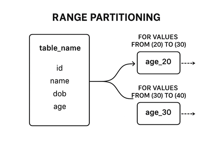
Range Partitioning

Here we create a partition on column while creating a table in db , with the values in column by specifing the range of that column we create a partitions.

Command:

Create table students ( 

id SERIAL Primary key, 

name VARCHAR, 

dob date, 

age integer) PARTITION BY RANGE (age) 

Create table age_20  PARTITION OF table_name FOR VALUES FROM  20 TO 30 

Create table age_30  PARTITION OF table_name FOR VALUES FROM  30 TO 40 

Here we are clustering the records on basis of age groups,here if we try to insert any records into table it goes and sits in their respective cluster. 
 
Have you got doubt that ‘ what happens when the retrivals are from various partions? ’ -- Here partition puring(parallel retrival of records from multiple partitions) comes into picture. 

For example : - 

Select name,age from  students where age between 25 to 30 
 
Here database paralllely gets the result 25-30 records from the age_20 and 30-35 from age_30 and returns the results.

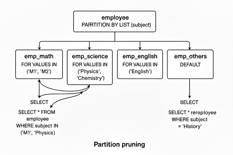
List Partitioning

We go for list partitioning when we have to partition the table based on a list of values in a field instead of mentioning the range of values of the field here we give provide the list of values.

Command:

Create table employee( 
		emp_id SERIAL Primary Key, 

emp_name VARCHAR, 

dept_id INTEGER, 

subject VARCHAR) PARTITION BY LIST (subject) 

Create table emp_math PARTITION OF employee 

    FOR VALUES IN ('M1',’M2); 

Create table emp_science PARTITION OF employee 

    FOR VALUES IN ('Physics',’Chemistry’); 

Create table emp_english PARTITION OF employee 

    FOR VALUES IN ('English'); 

Create table emp_others PARTITION OF employee DEFAULT 

 
Example : 
1. Select * from employee where subject in (‘M1’,’Physics’) 
 
	Here it goes parallel searching (partition pruning) gets applied on both partitions emp_math and emp_science . 
 

2. Select * from employee where subject = ‘History’

When these type of searches happen,which has no partition , those were stored in default partitin and that undergoes searching.If no default partition it raises an error.

Hash Partitioning

In Hash partitioning, data is distributed evenly by applying a hash function on a column (such as an ID or primary key) and assigning rows to partitions using:

“hash(id / pk) % number_of_partitions”

We use this technique when a table contains billions of rows, where other partitioning methods like range or list may not work efficiently.
By hashing on the ID, we can create multiple partitions upfront, which helps maintain balanced data distribution and ensures better performance.

Additionally, we can combine range and hash partitioning (known as composite partitioning) to achieve even more efficient data organization and query performance.

Command:

Create table orders ( 

    order_id BIGSERIAL PRIMARY KEY, 

    customer_id INT, 

    amount DECIMAL 

) PARTITION BY HASH (order_id); 

Create table orders_p0 PARTITION OF orders 

    FOR VALUES WITH (MODULUS 4, REMAINDER 0); 

Create table orders_p1 PARTITION OF orders 

    FOR VALUES WITH (MODULUS 4, REMAINDER 1); 

Create table orders_p2 PARTITION OF orders 

    FOR VALUES WITH (MODULUS 4, REMAINDER 2); 

Create table orders_p3 PARTITION OF orders 

    FOR VALUES WITH (MODULUS 4, REMAINDER 3)

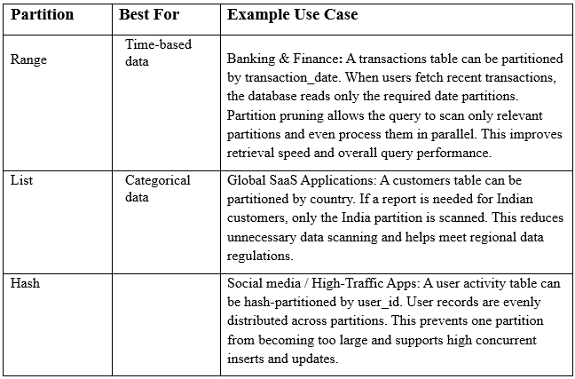
Best Use Cases

Key Takeaways

Table partitioning is a powerful optimization technique that makes querying large datasets faster by dividing a big table into smaller, manageable partitions.

The database still treats the partitioned table as a single logical table, so queries remain simple while performance improves.

Types of Partitioning:

Range Partitioning:

Data is divided based on continuous ranges (e.g., age groups 20–30, 30–40).

List Partitioning:

Data is grouped by discrete values (e.g., subjects like Math, Physics, English).

Hash Partitioning:

Data is evenly spread using a hash function, ideal for very large tables with billions of rows.

Partition Pruning:

Queries automatically retrieve data only from relevant partitions, enabling faster access and parallel processing.

A default partition can be defined to catch values that don’t fall into existing ranges or lists, preventing errors.

Composite partitioning (e.g., combining range + hash) can further optimize storage and query performance.

Use partitioning when tables grow very large, queries become slow, and you need efficient scalability.